Numerical methods for quantum time evolution

I recently took a course on Computational Physics and thought that playing with some of the methods would be a fun way to learn to use the Julia programming language. My idea was to reproduce some of the cool quantum time-evolution animations (see below) by applying numerical methods to the time-dependent Schrödinger equation.

This post contains nothing groundbreaking or especially cool, it’s essentially just playing around and having fun with some equations in Julia. Some of the goals of this experiment / exercise were:

1. Get familiar with Julia programming language
2. Get (more) familiar with numerical methods for solving partial differential equations.
3. Produce pretty animations of quantum systems evolving in time.
4. Improve my intuition about quantum time evolution and the Schrödinger equation.

Theory part: Schrödinger equation #

In quantum mechanics the state of the system is specified by wavefunction $\Psi$. For a 1-dimensional system (single particle in 1-D) $\Psi(x)$ is a function from real numbers to complex numbers. One postulate of quantum mechanics is that the time-evolution of quantum systems follows the Schrödinger equation

$$ i\hbar\frac{\dd\Psi}{\dd t} = H\Psi$$ where $H$ is the Hamiltonian operator. Such operators can be thought as functions over functions: if $\Psi$ is a function from $\R$ to $\C$, $H\Psi$ is also a function from $\R$ to $\C$. In our simple 1-dimensional case $H$ is defined as $$ H = -\frac{\hbar^2}{2 m}\frac{\dd}{\mathrm{d}x^2} + V(x)$$ where $V(x)$ is the potential energy, $m$ the mass of the particle and $\hbar$ the reduced Planck constant. This means \[ (H\Psi)(x) = -\frac{\hbar^2}{2 m}\frac{\dd\Psi(x)}{\mathrm{d}x^2} + V(x)\Psi(x) \]

The problem we’re interested in is the initial value problem: given wavefunction $\Psi(x, t=0)$, find wavefunction $\Psi(x,t)$. The approach is to consider tiny increments in time $\Delta t$: \[ \begin{aligned} \Psi(x, t+\Delta t) &\approx \Psi(x, t) + \frac{\Delta t}{i\hbar}H \Psi(x, t) \\ &= (1 + \frac{\Delta t}{i\hbar}H)\Psi(x, t) \end{aligned} \] As $\Delta t$ goes to zero the number of required steps $N=t/\Delta t$ goes to infinity. This gives us the solution of $\Psi(x,t)$ at arbitrary time \[ \begin{aligned} \Psi(x, t) &= \lim_{N\to\infty}\left(1 + \frac{t}{iN\hbar}H \right)^N\Psi(x, 0) \end{aligned} \] It turns out the above can be also written as \[ \begin{aligned} \Psi(x, t) &= \exp(\frac{itH}{\hbar}), \end{aligned} \] matching the limit definition of exponential function for real numbers: \[ \begin{aligned} \exp(x) &= \lim_{n\to\infty}\left(1+\frac{x}{n}\right)^n. \end{aligned} \] Understanding the exponentiation of operators is not really in the scope of this post though.

Discretization #

Since computers can’t work with infinite-dimensional spaces such as the space of functions $\R \to \C$, we need to discretize the wavefunction $\Psi$. In our case this means we select a range of $N$ evenly-spaced values for $x$ and represent $\Psi$ as a vector of $N$ complex numbers. We’ll denote the chosen positions as $x_i$ and the distance between two such points as $\Delta x = x_{i+1}-x_i$.

If you’re more at home with code than math, here’s the definition of $x$ and $\Psi$ in Julia:

L = 100  # The simulated line goes from -L/2 to L/2
N = 400
x = LinRange(-L/2, L/2, N)
# (In Julia it's normal to use unicode symbols)
# We'll be dealing with gaussian wave packets. More on that later.
Ψ = gaussian_wave_packet(0, 0, 1, x)  # See full source for details

We must also discretize the Hamiltonian operator $H$. In the discrete world, operators such as $H$ are represented by matrices. In this case $H$ is an $N$-by-$N$ matrix of complex numbers. To define this we must first discretize the operator $\frac{\dd^2}{\dd x^2}$.

Finite difference formula for $\frac{\dd^2}{\dd x^2}$ #

To define the operator $\frac{\dd^2}{\dd x^2}$ in matrix form we’re using the method of finite differences. The derivative of a function is defined as \[ \frac{\dd f(x)}{\dd x} =f^\prime(x)= \lim_{h \to 0} \frac{f(x+h)+f(x)}{h}. \] Numerically we can approximate the derivative with a discrete step $\Delta x$ in either positive or negative direction: \[ \begin{aligned} f^\prime(x) &\approx \frac{f(x + \Delta x) - f(x)}{\Delta x} \\ f^\prime(x) &\approx \frac{f(x) - f(x - \Delta x)}{\Delta x} \end{aligned} \] Applying these formulas twice we get an approximation formula for the second derivative $f^{\prime\prime}(x)$: \[ \begin{aligned} f^{\prime\prime}(x) &\approx \frac{f^\prime(x) - f^\prime(x - \Delta x)}{\Delta x} \\ &\approx \frac{ \frac{f(x+\Delta x)-f(x)}{\Delta x} - \frac{f(x)-f(x-\Delta x)}{\Delta x} }{\Delta x} \\ &\approx \frac{f(x+\Delta x)+f(x-\Delta)-2f(x)}{\Delta x^2}. \end{aligned} \]

For a discrete approximation of a function where $f_i=f(x_i)$ we can compute the second derivative of such representations easily: \[ f^{\prime\prime}(x_i) \approx \frac{1}{\Delta x^2}(x_{i+1}+x_{i-1}-2x_i). \] This can be represented as a matrix \[ D = \frac{1}{\Delta x^2} \begin{bmatrix} -2 & 1 & 0 & \ldots \\ 1 & -2 & 1 & \ldots \\ 0 & 1 &-2 & \ldots \\ 0 & 0 & 1 & \ldots \\ \vdots & \vdots & \vdots & \ddots \end{bmatrix}. \] Matrices like this which only have nonzero values along the main diagonal and the diagonals next to the main diagonal are called tridiagonal matrices.

While the math may look a bit complicated, the code in Julia is very simple:

L = 4
N = 400
x = LinRange(-L/2, L/2, N)
Δx = x[2] - x[1]
# SymTridiagonal is a special matrix type in Julia for symmetric
# tridiagonal matrices.
D2 = SymTridiagonal(-2 * ones(N), ones(N - 1)) / Δx^2
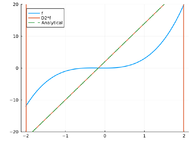
# Simple polynomial of third degree.
f = x.^2 + 2*x.^3
# Analytical solution to d²f/dx² for comparison
d2_f = 2 .+ 12 * x 
p = plot(x, [f D2*f d2_f],
    labels=["f" "D2*f" "Analytical"],
    ylim=(-20, 20),
    linestyle=[:solid :solid :dash],
    linewidth=2)
savefig(p, "d2.png")

Using this D2 we can now define the Hamiltonian matrix for the case of a free particle (potential $V(x)=0$). We’re using atomic units, meaning the electron mass $m$ and reduced Planck constant $\hbar$ have the value 1 (a.u).

const ħ = 1
const mass = 1

# Free particle hamiltonian:
H = -(ħ^2 / (2 * mass)) * D2

If we wanted to also include a nonzero potential, we need to add a matrix $W$ such that \[ (W\Psi)_i = V(x_i)\Psi_i. \] This can be done using a diagonal matrix. In Julia:

H = -(ħ^2 / (2 * mass)) * D2 + Diagonal(V(x))

Like SymTridiagonal, Diagonal is a special matrix type in Julia. Adding together a SymTridiagonal and Diagonal results in a SymTridiagonal matrix. This allows Julia to use faster algorithms for matrix-vector multiplication and linear system solving: $O(n)$ instead of $O(n^3)$ in the general (dense matrix) case.

Numerical methods #

Now that we’ve formalized the problem in matrix form, we’re looking to solve the initial value problem) of the following differential equation: \[ \frac{\dd \Psi}{\dd t} = \frac{1}{i\hbar} H\Psi \] Now $\Psi$ is just a vector of complex numbers and $H$ is a matrix (of reals in this case). The general idea is to discretize time into short steps of duration $\Delta t$.

To make following algorithm descriptions more general, we define a new matrix $F=H/i\hbar$. The algorithms below can then be used to solve any differential equation in the form \[ \frac{\dd \vec{y}}{\dd t} = F\vec{y}, \] where $\vec{y}$ is a vector of N numbers and $F$ is an N-by-N matrix.

Forward Euler #

Forward Euler method (or just simply Euler method) is the simplest way of solving initial value problems. It is derived from the finite difference approximation of the time derivative: \[ \begin{aligned} \frac{\dd \vec{y}}{\dd t} &= F\vec{y}(t) \\ &\approx \\ \frac{\vec{y}(t+\Delta t) - \vec{y}(t)}{\Delta t} &= F \vec{y}(t) \\ \vec{y}(t+\Delta t) &= \vec{y}(t)+{\Delta t} F \vec{y}(t) \end{aligned} \]

Code in Julia:

"""
    forward_euler(y, F, T, Δt)

Uses the Euler method to solve the initial value problem of differential
equation
  dy/dt = F * y
where y is a vector and F is a square matrix. Runs from time 0 to time T in
time steps of Δt. Returns a matrix with values of y after each step as columns.
"""
function forward_euler(y, F, T, Δt)
    steps = round(Int, T / Δt)
    # Make a matrix of size (length(y), steps)
    ys = similar(y, eltype(y), length(y), steps)
    U = I + Δt * F
    for i ∈ 1:steps
        y = U * y
        ys[:, i] = y
    end
    return ys
end

Backwards-Euler #

Backward Euler is a method similar to the one just described, except it uses a different finite-difference approximation: \[ \begin{aligned} \frac{\vec{y}(t+\Delta t) - \vec{y}(t)}{\Delta t} &= F \vec{y}(t+\Delta t). \\ \end{aligned} \] Here on the right side of the equation we’re evaluating $y$ at time $t+\Delta t$ instead of at $t$ like in the forward Euler. Now to solve for the new value of $y(t+\Delta t)$ we move all $y(t+\Delta t)$ to the left side of the equation and all $y(t)$ to the right side: \[ \begin{aligned} y(t+\Delta t)- y(t) &= \Delta t F y(t+\Delta t) \\ (I-\Delta t F) y(t+\Delta t) &= y(t). \end{aligned} \] The solution for $y(t+\Delta t)$ can be found by inverting the matrix: \[ y(t+\Delta t) = (I-\Delta t F)^{-1}y(t). \] In practice instead of matrix inverse we’ll be solving the linear system $(I-\Delta t F)\vec{y}^{(n)} = \vec{y}^{(n-1)} $.

Code:

function backward_euler(y, F, T, Δt)
    steps = round(Int, T / Δt)
    ys = similar(y, eltype(y), length(y), steps)
    # Julia defines I as a special identity matrix type, which is convenient
    # and allows for nice optimizations under the hood.
    L = I - Δt * F
    # Factorizing the matrix once and reusing this factorization makes
    # the following matrix division (A\b, solving A*x=b) much faster.
    # Since L ends up being a symmetric tridiagonal matrix, Julia knows to
    # use LDLᵀ-decomposition which performs this division in linear time.
    L_fac = factorize(L)
    for i ∈ 1:steps
        y = L_fac \ y
        ys[:, i] = y
    end
    return ys
end

Crank-Nicolson #

Another variation on Euler method is to take the average of forward Euler and backward Euler update. More formally, we’re using the finite difference approximation \[ \begin{aligned} \frac{\vec{y}(t+\Delta t) - \vec{y}(t)}{\Delta t} &= \frac{ F \vec{y}(t)+ F \vec{y}(t+\Delta t) }{2}. \end{aligned} \] Like in backward Euler, separate $\vec{y}(t)$ and $\vec{y}(t+\Delta t)$, arriving at \[ \begin{aligned} (I-\frac{1}{2}\Delta t F) y(t+\Delta t) &= (I+\frac{1}{2}\Delta t F) y(t) \end{aligned} \]

This is called the Crank-Nicolson method. Julia code is again quite simple:

function crank_nicolson(y, F, T, Δt)
    steps = round(Int, T / Δt)
    ys = similar(y, eltype(y), length(y), steps)
    A = Δt * F / 2
    L = I - A
    R = I + A
    L_fac = factorize(L)
    for i ∈ 1:steps
        y = L_fac \ (R * y)
        ys[:, i] = y
    end
    return ys
end

Comparison #

Below we see animations of each method with a few values for $\Delta t$ and $\Delta x$.

We see that forward Euler method blows up unless we select a small enough timestep ($\Delta t=0.001$). Backward Euler seems more stable, but “shrinks” over time. The norm displayed in the animations is defined as \[ ||\Psi|| = \left(\int_{-\infty}^\infty |\Psi(x)|^2 dx \right)^{1/2}. \] (In quantum mechanics the wavefunctions are almost always selected such that their norm is 1.)

Out of these methods, Crank-Nicolson is clearly the most suited method for this particular task. It also has the very nice property that the norm of the wavefunction is preserved.

Unitary matrices – Why did Crank-Nicolson preserve norm? #

Unitary matrix is a matrix which satisfies \[ U^\dag U = I, \] where $U^\dag$ is the conjugate transpose of $U$. In other words, $U^\dag = U^{-1}$ for unitary matrices. Conjugate transpose of matrix $U$ is obtained by transposing the matrix and taking the complex conjugate of each element. For example: \[ \begin{bmatrix} 1 & i \\ 1+2i & 1-i \end{bmatrix}^\dag = \begin{bmatrix} 1 & 1-2i \\ -i & 1+i \end{bmatrix}. \] An important feature of unitary matrices is that they preserve the length (norm) of vectors: $||U\vec{x}|| = ||\vec{x}||$. Some important unitary matrices are the identity matrix I and rotation matrices used to rotate vectors around an axis. Unitary matrices (and unitary operators) can be thought of as a generalization of the concept of rotation.

It turns out that the matrix representing a single step of the Crank-Nicolson method is unitary when we substitute $F=\frac{1}{2i m}H=-\frac{i}{2m}H$: \[ U = \left(I + \frac{\Delta t i}{2 m} H\right)^{-1} \left(I - \frac{\Delta t i}{2 m} H\right). \] We can see this by using the following properties of the conjugate transpose:

1. $(AB)^\dag = B^\dag A^\dag$
2. $(A+B)^\dag = A^\dag + B^\dag$
3. $(A^{-1})^\dag = (A^\dag)^{-1} = A^{-\dag}$
4. $(zA)^\dag = \bar{z}A^\dag$ where $\bar{z}$ is the complex conjugate of $z$
5. $I^\dag = I$ for the identity matrix $I$

\[ \begin{aligned} U^\dag &= \left( \left(I + \frac{\Delta t i}{2 m} H\right)^{-1} \left(I - \frac{\Delta t i}{2 m} H\right) \right)^\dag \\ &= \left(I - \frac{\Delta t i}{2 m} H\right)^\dag \left(I + \frac{\Delta t i}{2 m} H\right)^{-\dag} \\ &= \left(I^\dag - \left(\frac{\Delta t i}{2 m} H\right)^\dag\right) \left(I^\dag + \left(\frac{\Delta t i}{2 m} H\right)^\dag\right)^{-1} \\ &= \left(I + \frac{\Delta t i}{2 m} H^\dag\right) \left(I - \frac{\Delta t i}{2 m} H^\dag\right)^{-1} \end{aligned} \] Now recall that our $H$ was real and symmetric, meaning $H^\dag = H$. More generally, any Hamiltonian $H$ satisfies $H^\dag=H$ - this is the definition of a Hermitian operator a very important concept in quantum mechanics. Applying this property we get \[ \begin{aligned} U^\dag &= \left(I + \frac{\Delta t i}{2 m} H\right) \left(I - \frac{\Delta t i}{2 m} H\right)^{-1}. \end{aligned} \] This is the inverse of $U$: \[ \begin{aligned} U^\dag U &= \left(I + \frac{\Delta t i}{2 m} H\right) \left(I - \frac{\Delta t i}{2 m} H\right)^{-1} \left(I - \frac{\Delta t i}{2 m} H\right) \left(I + \frac{\Delta t i}{2 m} H\right)^{-1} \\ &= I. \end{aligned} \]

This property of norm preservation when applied to the Schrödinger equation makes Crank-Nicolson method particularly well-suited for time-evolution of quantum systems.

Cool animations #

Now that we’ve covered the methods and some theory it’s finally time to apply Crank-Nicolson to generate some cool animations of quantum behavior.

Conclusions / Future improvements #

I found writing numerical code in Julia to be a joy. The language is very well designed for these sorts of problems. I’m looking forward to doing more stuff Julia.

While Crank-Nicolson is clearly better at this task than the other methods explored here, it’s not perfect. Comparing the methods for moving particles shows that the shape of the wave packet gets distorted quite a lot with Crank-Nicolson compared to the exact analytical solution (copied from Shankar’s Principles of Quantum Mechanics, see code for details).

Some ideas for future exploration/improvement:

• Use finite element method, possibly using a FEM library like gridap.
• Two dimensions: simulate and visualize the double-slit experiment.
• Look up solutions or try to solve some of these simple but non-trivial cases analytically.

Source #

Julia source for generating all the figures and animations in this post can be found here.